Step 1. Integrate public and disease-specific datasets to train TriMap
Applying AI to biological questions often hinges on the availability of large, high-quality datasets. However, in many immunological contexts, such as modeling TCR–peptide–HLA (T-P-H) interactions, data are extremely limited, both in scale and specificity. As a result, models trained on one dataset often fail to generalize across diseases.
In this study, we demonstrate that integrating minimal task-specific data and large-scale data from unrelated diseases (e.g., viral infections) can significantly enhance model performance on a new disease. Specifically, we show that with just 39 peptides and 5 TCR binding measurements from ankylosing spondylitis (AS) patients, the model’s performance on AS-related prediction tasks improves from ineffective to highly usable. This approach highlights a promising strategy to overcome data scarcity in disease-specific TCR modeling.
Load required libraries
import pandas as pd
from trimap import utils
from trimap.model import TCRbind
import torch
import numpy as np

import warnings
warnings.filterwarnings("ignore")

seed = 0
np.random.seed(seed)
torch.manual_seed(seed)
torch.cuda.manual_seed(seed)
torch.cuda.manual_seed_all(seed)
torch.backends.cudnn.benchmark = False
torch.backends.cudnn.deterministic = True
device = torch.device("cuda:0" if torch.cuda.is_available() else "cpu")
Load training and validation datasets
The TCR sequences should be in the form of CDR3 regions, and the V and J gene information should be provided separately. All V and J genes should be in the Allele column of the trajs_aa.tsv, trajs_aa.tsv, trbjs_aa.tsv, and trbjs_aa.tsv. in the ‘library/’ folder.
Load the large-scale public VDJdb dataset
df_train = pd.read_csv('VDJdb.csv')
print(df_train.iloc[0])
alpha                                                  CIVRAPGRADMRF
beta                                            CASSYLPGQGDHYSNQPQHF
HLA                                                      HLA-B*08:01
Epitope                                                     FLKEKGGL
Epitope species                                                HIV-1
MHC class                                                       MHCI
V_alpha                                                  TRAV26-1*01
J_alpha                                                    TRAJ43*01
V_beta                                                     TRBV13*01
J_beta                                                    TRBJ1-5*01
Species                                                  HomoSapiens
Score                                                              2
Method             {"frequency": "", "identification": "tetramer-...
Name: 0, dtype: object
Reconstruct full TCR sequences by CDR3 and VJ gene information
df_train['alpha'] = utils.determine_tcr_seq_vj(df_train['alpha'].tolist(), df_train['V_alpha'].tolist(), df_train['J_alpha'].tolist(), chain='A')
df_train['beta'] = utils.determine_tcr_seq_vj(df_train['beta'].tolist(), df_train['V_beta'].tolist(), df_train['J_beta'].tolist(), chain='B')
df_train = df_train[['alpha', 'beta', 'V_alpha', 'J_alpha', 'V_beta', 'J_beta', 'HLA', 'Epitope']]
print(df_train.iloc[0])
alpha      DAKTTQPPSMDCAEGRAANLPCNHSTISGNEYVYWYRQIHSQGPQY...
beta       AAGVIQSPRHLIKEKRETATLKCYPIPRHDTVYWYQQGPGQDPQFL...
V_alpha                                          TRAV26-1*01
J_alpha                                            TRAJ43*01
V_beta                                             TRBV13*01
J_beta                                            TRBJ1-5*01
HLA                                              HLA-B*08:01
Epitope                                             FLKEKGGL
Name: 0, dtype: object
Load a small amount of disease-specific data
Experimentally validated immmunogenic peptides from yeast display that can be presented by HLA-B27 and activate TRBV9 T cells. Download AS_synthetic.csv
AS_synthetic = pd.read_csv('AS_synthetic.csv')
AS_synthetic['alpha'] = utils.determine_tcr_seq_vj(AS_synthetic['alpha'].tolist(), AS_synthetic['V_alpha'].tolist(), AS_synthetic['J_alpha'].tolist(), chain='A')
AS_synthetic['beta'] = utils.determine_tcr_seq_vj(AS_synthetic['beta'].tolist(), AS_synthetic['V_beta'].tolist(), AS_synthetic['J_beta'].tolist(), chain='B')
print(AS_synthetic.iloc[0])
Epitope                                            SRIMLLAPK
alpha      KQEVTQIPAALSVPEGENLVLNCSFTDSAIYNLQWFRQDPGKGLTS...
beta       DSGVTQTPKHLITATGQRVTLRCSPRSGDLSVYWYQQSLDQGLQFL...
HLA                                              HLA-B*27:05
label                                                      1
V_alpha                                            TRAV21*01
J_alpha                                            TRAJ21*01
V_beta                                              TRBV9*01
J_beta                                            TRBJ2-3*01
Name: 0, dtype: object
Load validation data
Experimentally validated eptiopes from microbial strains or human proteins that can be presented by HLA-B27 and activate TRBV9 T cells. Download AS_natural.csv
AS_natural = pd.read_csv('AS_natural.csv')
AS_natural['alpha'] = utils.determine_tcr_seq_vj(AS_natural['alpha'].tolist(), AS_natural['V_alpha'].tolist(), AS_natural['J_alpha'].tolist(), chain='A')
AS_natural['beta'] = utils.determine_tcr_seq_vj(AS_natural['beta'].tolist(), AS_natural['V_beta'].tolist(), AS_natural['J_beta'].tolist(), chain='B')
print(AS_natural.iloc[0])
alpha           KQEVTQIPAALSVPEGENLVLNCSFTDSAIYNLQWFRQDPGKGLTS...
beta            DSGVTQTPKHLITATGQRVTLRCSPRSGDLSVYWYQQSLDQGLQFL...
V_alpha                                                 TRAV21*01
J_alpha                                                 TRAJ28*01
V_beta                                                   TRBV9*01
J_beta                                                 TRBJ2-3*01
HLA                                                   HLA-B*27:05
Name                                                        AS3.1
Epitope                                                 TRLALIAPK
Epitope_name                                                PRPF3
label                                                           1
Name: 0, dtype: object
Warning
Note on model usage and evaluation
For validation purposes, we currently split the available data into training and testing sets. However, in real-world applications, both AS_synthetic.csv and AS_natural.csv should be included in the training set to achieve better predictive performance.
In addition, to mitigate potential variance due to random initialization, we recommend training the model under 10 different random seeds and aggregating the predictions from all runs (e.g., via ensembling) to obtain more stable and reliable results.
Training and saving the model
Train the model using the integrated dataset, which includes both the large-scale public VDJdb data and the small disease-specific data.
THEmodel = TCRbind().to(device)
THEmodel.train_model(df_train, df_add=AS_synthetic, num_epochs=20, device=device, phla_model_dir='phla_model.pt')
torch.save(THEmodel.state_dict(), 'TriMap_model_AS.pth')
INFO:trimap.model:Training...
You are using the default legacy behaviour of the <class 'transformers.models.t5.tokenization_t5.T5Tokenizer'>. This is expected, and simply means that the `legacy` (previous) behavior will be used so nothing changes for you. If you want to use the new behaviour, set `legacy=False`. This should only be set if you understand what it means, and thoroughly read the reason why this was added as explained in https://github.com/huggingface/transformers/pull/24565
INFO:trimap.model:Loading alpha_dict.pt
INFO:trimap.model:Found new alpha sequences, embedding...
100%|██████████| 3/3 [00:10<00:00,  3.59s/it]
INFO:trimap.model:Updated and saved alpha_dict.pt
INFO:trimap.model:Loading beta_dict.pt
INFO:trimap.model:Found new beta sequences, embedding...
100%|██████████| 3/3 [00:10<00:00,  3.63s/it]
INFO:trimap.model:Updated and saved beta_dict.pt
100%|██████████| 308/308 [01:45<00:00,  2.92it/s]
Epoch [1/20], Loss: 0.6157, ROC: 0.6784
100%|██████████| 308/308 [01:45<00:00, 2.91it/s]
Epoch [2/20], Loss: 0.5217, ROC: 0.7485
100%|██████████| 308/308 [01:56<00:00, 2.64it/s]
Epoch [3/20], Loss: 0.5745, ROC: 0.7776
100%|██████████| 309/309 [01:47<00:00, 2.87it/s]
Epoch [4/20], Loss: 0.4475, ROC: 0.7931
100%|██████████| 309/309 [01:39<00:00, 3.12it/s]
Epoch [5/20], Loss: 0.5160, ROC: 0.8059
100%|██████████| 308/308 [01:51<00:00, 2.77it/s]
Epoch [6/20], Loss: 0.4794, ROC: 0.8168
100%|██████████| 309/309 [01:48<00:00, 2.86it/s]
Epoch [7/20], Loss: 0.4577, ROC: 0.8276
100%|██████████| 309/309 [01:52<00:00, 2.75it/s]
Epoch [8/20], Loss: 0.4871, ROC: 0.8352
100%|██████████| 309/309 [01:51<00:00, 2.76it/s]
Epoch [9/20], Loss: 0.5085, ROC: 0.8454
100%|██████████| 309/309 [01:49<00:00, 2.83it/s]
Epoch [10/20], Loss: 0.4639, ROC: 0.8528
100%|██████████| 309/309 [01:43<00:00, 3.00it/s]
Epoch [11/20], Loss: 0.4757, ROC: 0.8632
100%|██████████| 308/308 [01:49<00:00, 2.82it/s]
Epoch [12/20], Loss: 0.3130, ROC: 0.8732
100%|██████████| 308/308 [01:32<00:00, 3.33it/s]
Epoch [13/20], Loss: 0.4456, ROC: 0.8788
100%|██████████| 309/309 [01:45<00:00, 2.94it/s]
Epoch [14/20], Loss: 0.3144, ROC: 0.8864
100%|██████████| 308/308 [01:33<00:00, 3.28it/s]
Epoch [15/20], Loss: 0.4011, ROC: 0.8964
100%|██████████| 308/308 [01:38<00:00, 3.12it/s]
Epoch [16/20], Loss: 0.3377, ROC: 0.9012
100%|██████████| 309/309 [01:42<00:00, 3.01it/s]
Epoch [17/20], Loss: 0.3542, ROC: 0.9097
100%|██████████| 308/308 [01:39<00:00, 3.08it/s]
Epoch [18/20], Loss: 0.3387, ROC: 0.9179
100%|██████████| 308/308 [01:38<00:00, 3.12it/s]
Epoch [19/20], Loss: 0.3592, ROC: 0.9235
100%|██████████| 309/309 [01:40<00:00, 3.07it/s]
Epoch [20/20], Loss: 0.4734, ROC: 0.9290
(optional) Load pretrained model
THEmodel = TCRbind().to(device)
THEmodel.load_state_dict(torch.load('TriMap_model_AS.pth', map_location=device))
<All keys matched successfully>
Validate the model on the validation dataset
Validate the model using the micribial or human protein-derived epitopes
result, alpha_attn, beta_attn = THEmodel.test_model(df_test=AS_natural, device=device, phla_model_dir='pHLA_model.pt')
AS_natural['pred'] = result
INFO:trimap.model:Loading alpha_dict.pt
INFO:trimap.model:No new alpha sequences found
INFO:trimap.model:Loading beta_dict.pt
INFO:trimap.model:No new beta sequences found
INFO:trimap.model:Predicting...
100%|██████████| 1/1 [00:00<00:00,  1.33it/s]
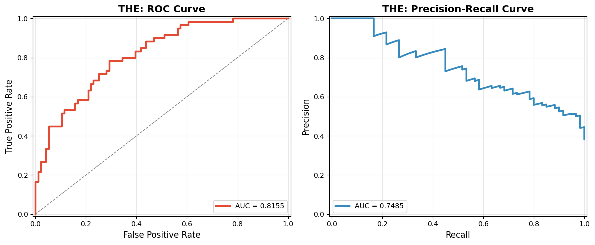
Plot AUROC and AUPRC curves
import matplotlib.pyplot as plt
from sklearn.metrics import (
    roc_curve,
    precision_recall_curve,
    roc_auc_score,
    average_precision_score
)

def plot_roc_prc_curve(y_true, y_scores, title_prefix=''):
    """
    Plot aesthetically improved ROC and Precision-Recall curves with AUC scores.

    Args:
        y_true (array-like): Ground truth binary labels (0 or 1).
        y_scores (array-like): Predicted scores (e.g., probabilities).
        title_prefix (str): Optional prefix for plot titles.
    """
    # Use a clean style
    plt.style.use('seaborn-v0_8-muted')

    # Compute metrics
    fpr, tpr, _ = roc_curve(y_true, y_scores)
    roc_auc = roc_auc_score(y_true, y_scores)

    precision, recall, _ = precision_recall_curve(y_true, y_scores)
    prc_auc = average_precision_score(y_true, y_scores)

    # Print AUC values
    print(f'{title_prefix}ROC-AUC: {roc_auc:.4f}')
    print(f'{title_prefix}PRC-AUC: {prc_auc:.4f}')

    # Set up plot
    fig, axes = plt.subplots(1, 2, figsize=(12, 5))

    # ROC Curve
    axes[0].plot(fpr, tpr, color='#E24A33', lw=2.5, label=f'AUC = {roc_auc:.4f}')
    axes[0].plot([0, 1], [0, 1], linestyle='--', color='gray', lw=1)
    axes[0].set_xlim([-0.01, 1.01])
    axes[0].set_ylim([-0.01, 1.01])
    axes[0].set_xlabel('False Positive Rate', fontsize=12)
    axes[0].set_ylabel('True Positive Rate', fontsize=12)
    axes[0].set_title(f'{title_prefix}ROC Curve', fontsize=14, fontweight='bold')
    axes[0].legend(loc='lower right', fontsize=10)
    axes[0].grid(alpha=0.3)

    # PRC Curve
    axes[1].plot(recall, precision, color='#348ABD', lw=2.5, label=f'AUC = {prc_auc:.4f}')
    axes[1].set_xlim([-0.01, 1.01])
    axes[1].set_ylim([-0.01, 1.01])
    axes[1].set_xlabel('Recall', fontsize=12)
    axes[1].set_ylabel('Precision', fontsize=12)
    axes[1].set_title(f'{title_prefix}Precision-Recall Curve', fontsize=14, fontweight='bold')
    axes[1].legend(loc='lower left', fontsize=10)
    axes[1].grid(alpha=0.3)

    plt.tight_layout()
    plt.show()

plot_roc_prc_curve(AS_natural['label'], AS_natural['pred'], title_prefix='THE: ')
THE: ROC-AUC: 0.8155
THE: PRC-AUC: 0.7485
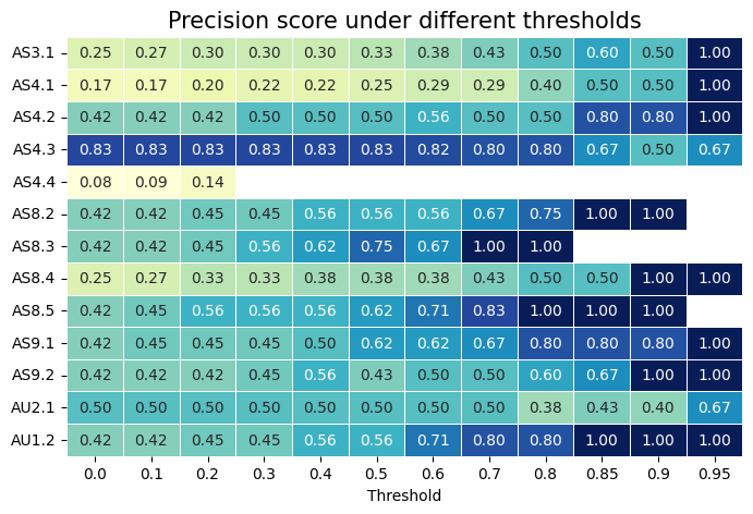
Calculate precision score under different thresholds
This indicates when the model is highly confident in its predictions, it is more likely to be correct.
from sklearn.metrics import confusion_matrix
import seaborn as sns
thresholds = [0.0, 0.1,0.2,0.3,0.4,0.5,0.6,0.7,0.8,0.85,0.9, 0.95]
tcr_unique = AS_natural['Name'].value_counts().index.tolist()
precision_all = []
for tcr in tcr_unique:
    precision_list = []
    for threshold in thresholds:
        df_baselines = AS_natural[AS_natural['Name'] == tcr]
        cm = confusion_matrix(df_baselines['label'].values, df_baselines['pred'].values > threshold)
        TP = cm[1, 1]
        FP = cm[0, 1]
        precision = TP / (TP + FP) if (TP + FP) > 0 else 0
        # precision = TP
        precision_list.append(precision)
    precision_all.append(precision_list)

# Create a DataFrame
df = pd.DataFrame(precision_all, columns=thresholds, index=tcr_unique)

# Create the heatmap
# if precision is 0, delete the value
df = df.replace(0, np.nan)
plt.figure(figsize=(8, 5))
sns.heatmap(df, cmap='YlGnBu', annot=True, fmt=".2f", linewidths=0.5, cbar=False)
plt.xlabel('Threshold')
plt.title('Precision score under different thresholds', fontsize=15)
#hidden colorbar
plt.show()
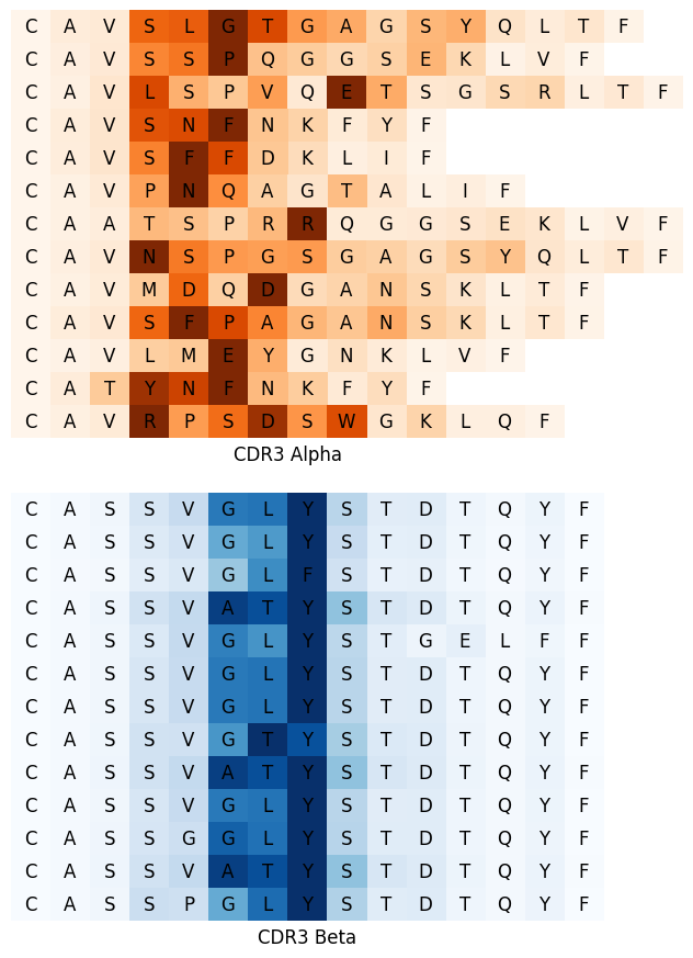
Visualize the attention weights for CDR3 regions
def find_alpha_region(seq):
    start = seq.find('CA')
    for tag in ['TF', 'IF', 'YF', 'VF', 'QF']:
        end = seq.find(tag)
        if end != -1:
            return start, end + 2
    return start, len(seq)

def find_beta_region(seq):
    start = seq.find('CA')
    for tag in ['TQYF', 'ELFF']:
        end = seq.find(tag)
        if end != -1:
            return start, end + len(tag)
    return start, len(seq)

def extract_cdr3_ab_pairs(alpha_seqs, beta_seqs, alpha_attn_tensor, beta_attn_tensor):
    out_alpha_seqs, out_alpha_attns = [], []
    out_beta_seqs, out_beta_attns = [], []

    for i in range(len(alpha_seqs)):
        a_start, a_end = find_alpha_region(alpha_seqs[i])
        b_start, b_end = find_beta_region(beta_seqs[i])
        if a_start != -1 and a_end > a_start and b_start != -1 and b_end > b_start:
            out_alpha_seqs.append(alpha_seqs[i][a_start:a_end])
            out_alpha_attns.append(alpha_attn_tensor[i][:, :, a_start:a_end])
            out_beta_seqs.append(beta_seqs[i][b_start:b_end])
            out_beta_attns.append(beta_attn_tensor[i][:, :, b_start:b_end])

    return out_alpha_seqs, out_alpha_attns, out_beta_seqs, out_beta_attns

def plot_cdr3_ab_attn_split(alpha_seq, alpha_attn, beta_seq, beta_attn, alpha_set, channels=(2,3,4,5,6,7)):

    max_len = max(
        max((len(seq) for seq in alpha_seq), default=1),
        max((len(seq) for seq in beta_seq), default=1)
    )

    width_per_aa = 0.4
    height_per_row = 0.3
    fig_height = len(alpha_set) * height_per_row * 2 + 1
    fig = plt.figure(figsize=(max_len * width_per_aa, fig_height))

    for i, seq in enumerate(alpha_set):
        idxs = [j for j, s in enumerate(alpha_seq) if s == seq]
        if not idxs:
            continue
        j = idxs[0]
        attn_a = alpha_attn[j][channels, :, :].sum((0, 1))  # shape: (seq_len,)
        attn_b = beta_attn[j][channels, :, :].sum((0, 1))
        seq_a = alpha_seq[j]
        seq_b = beta_seq[j]

        # --- alpha 行 ---
        ax1 = fig.add_axes([
            0.05,
            1 - (i + 1) * height_per_row / fig_height,
            len(seq_a) / max_len * 0.9,
            height_per_row / fig_height
        ])
        ax1.imshow(attn_a.unsqueeze(0).numpy(), aspect='auto', cmap='Oranges')
        for k, aa in enumerate(seq_a):
            ax1.text(k, 0, aa, ha='center', va='center', fontsize=12)
        ax1.set_xticks([]); ax1.set_yticks([])
        for spine in ax1.spines.values():
            spine.set_visible(False)
        ax1.set_xlabel('CDR3 Alpha', fontsize=12)

        # --- beta 行 ---
        ax2 = fig.add_axes([
            0.05,
            0.5 - (i + 1) * height_per_row / fig_height,
            len(seq_b) / max_len * 0.9,
            height_per_row / fig_height
        ])
        ax2.imshow(attn_b.unsqueeze(0).numpy(), aspect='auto', cmap='Blues')
        for k, bb in enumerate(seq_b):
            ax2.text(k, 0, bb, ha='center', va='center', fontsize=12)
        ax2.set_xticks([]); ax2.set_yticks([])
        for spine in ax2.spines.values():
            spine.set_visible(False)
        ax2.set_xlabel('CDR3 Beta', fontsize=12)

    plt.show()

pos_index = AS_natural[AS_natural['label'] == 1].index
alpha_seq = AS_natural.loc[pos_index, 'alpha'].values
beta_seq = AS_natural.loc[pos_index, 'beta'].values
alpha_attn_tensor = alpha_attn[pos_index]
beta_attn_tensor = beta_attn[pos_index]

alpha_seq, alpha_attn_cdr3, beta_seq, beta_attn_cdr3 = extract_cdr3_ab_pairs(
    alpha_seq, beta_seq, alpha_attn_tensor, beta_attn_tensor
)

alpha_set = [
    'CAVSLGTGAGSYQLTF','CAVSSPQGGSEKLVF','CAVLSPVQETSGSRLTF',
    'CAVSNFNKFYF','CAVSFFDKLIF','CAVPNQAGTALIF','CAATSPRRQGGSEKLVF',
    'CAVNSPGSGAGSYQLTF','CAVMDQDGANSKLTF','CAVSFPAGANSKLTF',
    'CAVLMEYGNKLVF','CATYNFNKFYF','CAVRPSDSWGKLQF'
]

plot_cdr3_ab_attn_split(alpha_seq, alpha_attn_cdr3, beta_seq, beta_attn_cdr3, alpha_set)